


Next: The vector nature of
Up: Electromagnetic Waves.
Previous: Sinusoidal Oscillations.
Contents
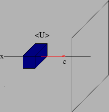
Figure 7.8:
 |
We now turn our attention to the energy carried by the electromagnetic
wave. For simplicity we shall initially restrict ourselves to points
located
along the  axis for the situation shown in Figure 7.7.
The energy density in the electric and magnetic fields is given
by
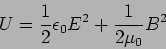 |
(7.18) |
For an electromagnetic wave the electric and magnetic fields are
related. The energy density can then be written in terms of only the
electric field as
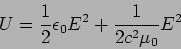 |
(7.19) |
The speed of light  is related to
  and
and  as
as
 . Using this we find that the energy density has
the form
. Using this we find that the energy density has
the form
 |
(7.20) |
The instantaneous energy density of the electromagnetic wave
oscillates with time. The time average of the energy density is often
a more useful quantity. We have already discussed how to calculate the
time average of an oscillating quantity. This is particularly simple
in the complex notation where the electric field
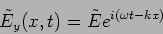 |
(7.21) |
has a mean squared value
 . Using this we
find that the average energy density is
. Using this we
find that the average energy density is
 |
(7.22) |
where  is the amplitude of the electric field.
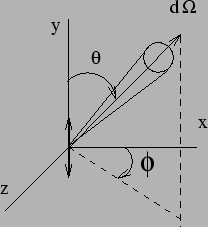
We next consider the energy flux of the electromagnetic
radiation. The radiation propagates along the axis at the point
where we want to calculate the flux. Consider a surface which is
perpendicular to direction in which the wave is propagating
as shown in Figure 7.8. The energy flux  refers to the
energy which crosses an unit area of this surface in unit time. It
has units
refers to the
energy which crosses an unit area of this surface in unit time. It
has units
 . The flux is the power that would be
received by collecting the radiation in an area
. The flux is the power that would be
received by collecting the radiation in an area  placed
perpendicular to the direction in which the wave is propagating
as shown in Figure 7.8.
placed
perpendicular to the direction in which the wave is propagating
as shown in Figure 7.8.
The average flux can be calculated by noting that the wave propagates along
the axis with speed . The average energy
 contained in an unit volume would take a time to cross the
surface. The flux is the energy which would cross in one second which
is
contained in an unit volume would take a time to cross the
surface. The flux is the energy which would cross in one second which
is
 |
(7.23) |
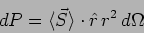
The energy flux is actually a vector quantity representing both the
direction and the rate at which the wave carries energy. Referring
back to equation (7.8) and (7.15) we see that
at any point the average flux
 is pointed
radially outwards and has a value
is pointed
radially outwards and has a value
 |
(7.24) |
Note that the flux falls as  as we move away from the
source. This is a property which may already be familiar to some of us
from considerations of the conservation of energy. Note that the total
energy crossing a surface enclosing the source will be constant
irrespective of the shape and size of the surface.
as we move away from the
source. This is a property which may already be familiar to some of us
from considerations of the conservation of energy. Note that the total
energy crossing a surface enclosing the source will be constant
irrespective of the shape and size of the surface.
Figure 7.9:
 |
Let us know shift our point of reference to the location of the dipole
and ask how much power is radiated in any given direction. This is
quantified using the power emitted per solid angle. Consider a solid
angle  along a direction
  at an angle
 to the dipole as shown in Figure 7.9. The power
 radiated into this solid angle can be calculated by multiplying the
flux with the area corresponding to this solid angle
radiated into this solid angle can be calculated by multiplying the
flux with the area corresponding to this solid angle
 |
(7.25) |
which gives us the power radiated per unit solid angle to be
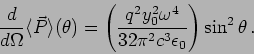 |
(7.26) |
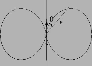
This tells us the radiation pattern of the dipole radiation,
ie.. the directional dependence of the radiation is proportional to
 . The radiation is maximum in the direction
perpendicular to the dipole while there is no radiation emitted
along the direction of the dipole. The radiation pattern is shown in
Figure 7.10. Another important point to note is that the
radiation depends on
. The radiation is maximum in the direction
perpendicular to the dipole while there is no radiation emitted
along the direction of the dipole. The radiation pattern is shown in
Figure 7.10. Another important point to note is that the
radiation depends on  which tells us that the same dipole
will radiate significantly more power if it is made to oscillate
at a higher frequency, doubling the frequency will increase the
power sixteen times.
which tells us that the same dipole
will radiate significantly more power if it is made to oscillate
at a higher frequency, doubling the frequency will increase the
power sixteen times.
Figure 7.10:
 |
The total power radiated can be calculated by integrating over all
solid angles. Using
 and
and
 |
(7.27) |
gives the total power  to be
to be
It is often convenient to express this in terms of the amplitude of
the current in the wires of the oscillator as
 |
(7.29) |
The power radiated by the electric dipole is proportional to the
square of the current. This behaviour is exactly the same as that of a
resistance except that the oscillator emits the power as radiation
while the resistance converts it to heat. We can express the radiated
power in terms of an equivalent resistance with
 |
(7.30) |
where
 |
(7.31) |
 being the length of the dipole (Figure 7.5) and
 the wavelength of the radiation.
Problems
- An oscillating current of amplitude
 and
and
 is fed into a dipole antenna of length
  oriented along the
  axis and located at
  . All
coordinates are in
. All
coordinates are in  and
and
 .
.
- a.
- What is the amplitude of the electric field at the point
 ? (
? (
 )
)
- b.
- In which direction does the electric oscillate at the point
? [Give the angles with respect to the , and
 axis.] (
 ,
,  ,
, 
- c.
- What is the total power radiated? (
 )
)
- d.
- How does the total power change if the frequency is doubled?
(
 times)
- A charge
 moves in a circular orbit with period
  in the
 plane with center at the origin . The charge is at
at
plane with center at the origin . The charge is at
at  , and the motion is counter-clockwise as seen
from the point P
, and the motion is counter-clockwise as seen
from the point P  where
where  . At a later time
- a.
- What is the acceleration of the charge?
- b.
- For the point P, what is the retarded acceleration of the
charge?
- c.
- What is the electric field at P?
- d.
- What is the time averaged power radiated by the charge?
- In which direction does an oscillating electric dipole radiate
maximum power? What is the FWHM of the radiation pattern?
- For the same peak current and frequency, how does the total power
change if the length of the dipole is halved.
- Consider a conducting wire of length
 and
and  diameter. At what frequency does the radiative resistance become
comparable to the usual Ohmic resistance. Use
diameter. At what frequency does the radiative resistance become
comparable to the usual Ohmic resistance. Use
 which is the typical value of conductivity for
conducting metals.
which is the typical value of conductivity for
conducting metals.
- An electric dipole oscillator radiates
 power. What
is the
flux
power. What
is the
flux  away in the direction perpendicular to the dipole
and at
away in the direction perpendicular to the dipole
and at  to the dipole.
- Particles of charge and mass
 with kinetic energy
are injected perpendicular to a magnetic field .
The charges experiences an acceleration as they go around in
circles in the magnetic field. Calculate the rate at which the
energy is radiated. Show that the energy of the particles falls
as
with kinetic energy
are injected perpendicular to a magnetic field .
The charges experiences an acceleration as they go around in
circles in the magnetic field. Calculate the rate at which the
energy is radiated. Show that the energy of the particles falls
as
 , where
  the decay time is related to
 and .
and .
Cyclotrons typically have magnetic fields of  or higher.
Using this value, calculate the frequency at which the radiation will
be emitted for electrons
or higher.
Using this value, calculate the frequency at which the radiation will
be emitted for electrons
 and protons
. Calculate for protons and electrons, and use
this to determine how long it will take for them to radiate away half
the initial kinetic energy.
and protons
. Calculate for protons and electrons, and use
this to determine how long it will take for them to radiate away half
the initial kinetic energy.
Next: The vector nature of
Up: Electromagnetic Waves.
Previous: Sinusoidal Oscillations.
Contents
Physics 1st Year
2009-01-06