We next consider a situation where a sinusoidal voltage is applied to
the dipole oscillator. The dipole is aligned with the
![]() axis (Figure 7.7). The voltage causes the charges to
move up and down as
axis (Figure 7.7). The voltage causes the charges to
move up and down as
It is often useful and interesting to represent the oscillating
charge in terms of other equivalent quantities namely the dipole
moment and the current in the circuit.
Let us replace the charge ![]() which moves up and down as by
two charges, one charge
which moves up and down as by
two charges, one charge ![]() which moves as
which moves as ![]() and another
charge
and another
charge ![]() which moves in exactly the opposite direction as
. The electric field produced by the new configuration
is exactly the same as that produced by the single charge considered
earlier. This allows us to interpret eq. (7.8) in terms of an
oscillating dipole
which moves in exactly the opposite direction as
. The electric field produced by the new configuration
is exactly the same as that produced by the single charge considered
earlier. This allows us to interpret eq. (7.8) in terms of an
oscillating dipole
which allows us to write eq. (7.8) as
Returning once more to the dipole oscillator shown in Figure
7.5, we note that the excess electrons which rush from A
to B when B has a positive voltage reside at the tip of the
wire B. Further, there is an equal excess of positive charge in A
which resides at the tip of A. The fact that excess charge resides at
the tips of the wire is property of charges on conductors which
should be familiar from the study of electrostatics. Now the dipole
moment is
![]() where
where ![]() is the length of the dipole
oscillator
and
is the length of the dipole
oscillator
and ![]() is the excess charge accumulated at one of the tips. This
allows us to write
is the excess charge accumulated at one of the tips. This
allows us to write ![]() in terms of the current in the
wires
in terms of the current in the
wires
![]() as
as
We now end the small detour where we discussed how the electric field
is related to the dipole moment and the current, and return to our
discussion of the electric field predicted by eq. (7.8).
We shall restrict our attention to points along the ![]() axis. The
electric field of the radiation is in the
axis. The
electric field of the radiation is in the ![]() direction and has a value
direction and has a value
Let us consider a situation where we are interested in the ![]() dependence of the electric field at a great distance from
the emitter. Say
we are
dependence of the electric field at a great distance from
the emitter. Say
we are ![]() away from the oscillator and we would like to know
how the electric field varies at two points which are
away from the oscillator and we would like to know
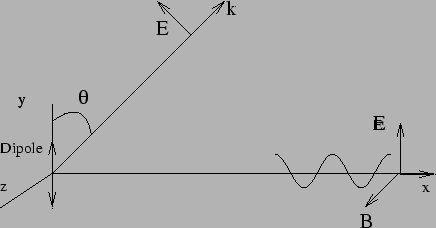
how the electric field varies at two points which are ![]() apart. This situation is shown schematically in Figure
7.7. The point to note is that a small variation in
apart. This situation is shown schematically in Figure
7.7. The point to note is that a small variation in ![]() will make a very small difference to the
will make a very small difference to the ![]() dependence of the
electric field which we can neglect, but the change in the
dependence of the
electric field which we can neglect, but the change in the ![]() term
cannot be neglected. This is because
term
cannot be neglected. This is because ![]() is multiplied by a factor
is multiplied by a factor
![]() which could be large and a change in
which could be large and a change in ![]() would mean a different phase of the oscillation. Thus at large distances
the electric field of the radiation can be well described by
would mean a different phase of the oscillation. Thus at large distances
the electric field of the radiation can be well described by
Although our previous discussion was restricted to points along the
![]() axis, the facts which we have learnt about the electric and
magnetic fields hold at any position (Figure 7.7).
At any point the direction of the electromagnetic wave is radially
outwards with wave vector
axis, the facts which we have learnt about the electric and
magnetic fields hold at any position (Figure 7.7).
At any point the direction of the electromagnetic wave is radially
outwards with wave vector
![]() . The electric and magnetic
fields are mutually perpendicular, they are also perpendicular to the
wave vector
. The electric and magnetic
fields are mutually perpendicular, they are also perpendicular to the
wave vector ![]() .
.
![\begin{displaymath}
E(t)=\frac{q y_0 \omega^2 }{4 \pi \epsilon_0 c^2 r} \,
\cos[ \omega (t-r/c)] \, \sin \theta \,.
\end{displaymath}](img571.png)
![\begin{displaymath}
E_y(x,t)=\frac{q y_0 \omega^2 }{4 \pi \epsilon_0 c^2 x} \,
\cos\left[ \omega t-\left(\frac{\omega}{c}\right) x \right]
\end{displaymath}](img585.png)