In Newtonian Mechanics the trajectory is determined by
solving Newton's equation of motion
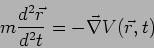 |
(20.1) |
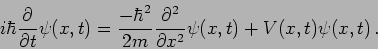
In Quantum Mechanics the wavefunction is governed by
Schrodinger's equation
For a particle free to move only in one dimension along the  axis we
have
axis we
have
 |
(20.3) |
Here we shall only consider time independent potentials  .
Applying the method of separation of variables we take a trial
solution
.
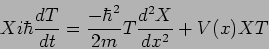
Applying the method of separation of variables we take a trial
solution
whereby the Schrodinger's equation is
 |
(20.5) |
which on dividing by  gives
gives
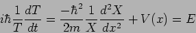 |
(20.6) |
The first term is a function of  alone whereas the second term is a
function of alone. It is clear that both terms must have a
constant value if they are to be equal for all values of and
. Denoting this constant as
alone whereas the second term is a
function of alone. It is clear that both terms must have a
constant value if they are to be equal for all values of and
. Denoting this constant as  we can write the solution for the time dependent part as
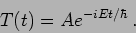 |
(20.7) |
The dependence has to be determined by solving
![\begin{displaymath}
\frac{\hbar^2}{2m}
\frac{d^2 X}{dx^2} = - [E-V(x)] X\,.
\end{displaymath}](img1565.png) |
(20.8) |
The general solution can be written as
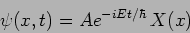 |
(20.9) |
where the dependence is known and  has to be determined from
equation (20.8).
has to be determined from
equation (20.8).
Free particle
The potential  for a free particle. It is straightforward to
verify that
for a free particle. It is straightforward to
verify that
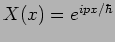 with
with
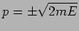 satisfies
equation (20.8).
This gives the solution
satisfies
equation (20.8).
This gives the solution
 |
(20.10) |
The is a plane wave with angular frequency
 and wave
number
and wave
number  where and
  are as yet arbitrary
constant related as
are as yet arbitrary
constant related as  . This gives the wave's dispersion
relation
. This gives the wave's dispersion
relation
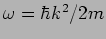 .
.
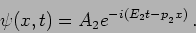
Here different value of will give different wavefunctions. For
example  and
and  are different constants with
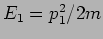 and
and 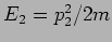 , then
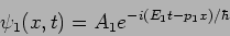 |
(20.11) |
and
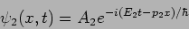 |
(20.12) |
are two different wavefunctions corresponding to two different states
of the particle.
What happens when we make a measurement?
We have already discussed what happens when we measure a particle's
position. In Quantum Mechanics it is not possible to predict
the particle's position. We can only predict probabilities for finding
the particle at different positions. The probability density
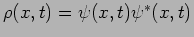 gives the probability
  of finding the particle in the interval
  around the point to
be
around the point to
be
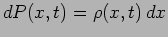 .
But there are other quantities like momentum which we could also
measure. What happens when we measure the momentum?
.
But there are other quantities like momentum which we could also
measure. What happens when we measure the momentum?
InQuantum Mechanics there is a Hermitian Operator
corresponding to every observable dynamical quantity like the
momentum, angular momentum, energy , etc.
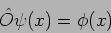
What is an operator? An operator  acts on a function
 to give another function
  .
.
 |
(20.15) |
We consider an example where

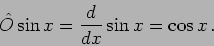 |
(20.16) |
Consider another example where  so that
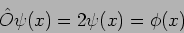 |
(20.17) |
What is a Hermitian operator? We do not go into the definition
here, instead we only state a relevant, important property of a
Hermitian operators. Given an operator  , a function
is an eigenfunction of with eigenvalue
, a function
is an eigenfunction of with eigenvalue
 if
if
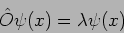 |
(20.18) |
As an example consider
 |
(20.19) |
we see that
 |
(20.20) |
The function  is an eigenfunction of the operator
 with eigenvalue
  .
As another example for the same operator we consider the
function
.
As another example for the same operator we consider the
function
 |
(20.21) |
we see that
 |
(20.22) |
This is not an eigenfunction of the operator.
Hermitian operators are a special kind of operators all of whose
eigenvalues are real.
We present the Hermitian operators corresponding to a few observable
quantities.
Position - x  Operator
 |
(20.23) |
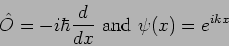
Momentum - p Operator 
 |
(20.24) |
Hamiltonian
 Operator
 |
(20.25) |
The eigenvalues of the Hamiltonian correspond to the
Energy.
Let us return to what happens when we make a measurement. Consider a
particle in a state with wavefunction  .
We measure its momentum . There are two possibilities
.
We measure its momentum . There are two possibilities
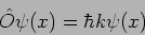
A. If is an eigenfunction of . For
example
 |
(20.26) |
 |
(20.27) |
We will get the value  for the momentum The measurement
does not disturb the state and after the measurement the particle
continues to be in the same state with wavefunction .
for the momentum The measurement
does not disturb the state and after the measurement the particle
continues to be in the same state with wavefunction .
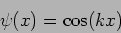
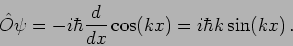
B. If is not an eigenfunction of . For
example
 |
(20.28) |
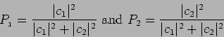
On measuring the momentum we will get either or  .
The probability of getting
is
.
The probability of getting
is
 and probability of getting
is
and probability of getting
is
 The measurement changes the wavefunction.
In case we get the wavefunction will be changed to
 |
(20.29) |
and in case we get - the wavefunction will be changed to
 |
(20.30) |
If we measure again we shall continue to get the same value in
every successive measurement.
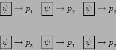
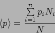
In general, if
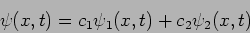 |
(20.31) |
such that
On measuring 
 |
(20.33) |
are are probabilities of getting the values  and
and  respectively.
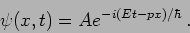
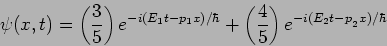
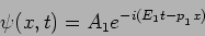
We can now interpret the solution
respectively.
We can now interpret the solution
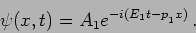 |
(20.34) |
This corresponds to a particle with momentum  and energy
 . We will get these value however many times we repeat the
measurement .
. We will get these value however many times we repeat the
measurement .
What happens if we measure the position of a particle whose
wavefunction is given by equation (20.34)?
Calculating the probability density
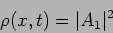 |
(20.35) |
we see that this has no dependence. The probability of finding the
particle is equal at all points. This wave function has no position
information.
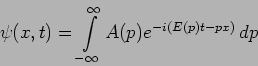
 .
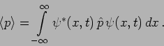
In Quantum Mechanics
it is possible to predict this using the particle's wavefunction as
.
In Quantum Mechanics
it is possible to predict this using the particle's wavefunction as