


Next: Phased array
Up: Diffraction
Previous: Angular resolution
Contents
Figure 12.10:
Chain of
coherent dipoles
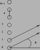 |
Consider N dipole oscillators arranged along a linear chain as
shown in Figure 12.10, all emitting radiation with
identical amplitude and phase. How much radiation will a distant
observer at an angle  receive? If
 are the
radiations from the
are the
radiations from the  th,
th,  st,
st,  nd, ...,and the
  th
oscillator respectively,
th
oscillator respectively,  is identical to
  except for a phase difference as it travels a shorter path. We
have
except for a phase difference as it travels a shorter path. We
have
 |
(12.12) |
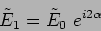
where
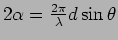 is the
phase difference that arises due to the path difference. Similarly
is the
phase difference that arises due to the path difference. Similarly
![$ \tilde E_2 = \left[ e^{i2 \alpha } \right]^2 \tilde E_0 $](img1001.png) . The
total radiation is obtained by summing the contributions from all
the sources and we have
. The
total radiation is obtained by summing the contributions from all
the sources and we have
![\begin{displaymath}
\tilde E =\sum \limits^{N-1}_{n=0} \tilde E_n =
\sum \limits^{N-1}_{n=0} \left[ e^{i 2 \alpha } \right]^n
\tilde E_0
\end{displaymath}](img1002.png) |
(12.13) |
This is a geometric progression, on summing this we have
 |
 |
|
(12.14) |
This can be simplified further
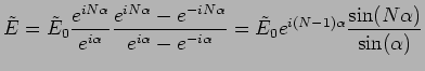 |
|
|
(12.15) |
which gives the intensity to be
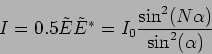 |
(12.16) |
where
 |
(12.17) |
Figure 12.11:
Intensity
pattern for chain of dipoles
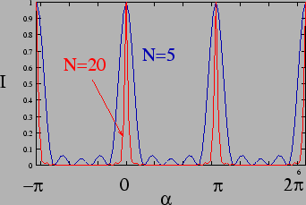 |
Plotting the intensity as a function of  (Figure 12.11) we see that it has a value
  at
at  . Further, it has the same value
  at all other values where both the numerator and
denominator are zero i.e
at all other values where both the numerator and
denominator are zero i.e
 or
or
 |
(12.18) |
The intensity is maximum whenever this condition is satisfied
These are referred to as the primary maxima of the diffraction
pattern and  gives the order of the maximum.
The intensity drops away from the primary maxima. The intensity
becomes zero times between any two successive primary
maxima and there are  secondary maxima in between. The
number of secondary maxima increases and the primary maxima
becomes increasingly sharper (Figure 12.11) if the
number of sources
secondary maxima in between. The
number of secondary maxima increases and the primary maxima
becomes increasingly sharper (Figure 12.11) if the
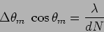
number of sources  is increased. Let us estimate the width of
the th order principal maximum. The th order principal
maximum occurs at an angle
is increased. Let us estimate the width of
the th order principal maximum. The th order principal
maximum occurs at an angle  which satisfies,
 |
(12.19) |
If
 is the width of the maximum, the intensity
should be zero at
is the width of the maximum, the intensity
should be zero at
 ie.
ie.
 |
(12.20) |
which implies that
 |
(12.21) |
Expanding
and assuming that
 we have
 |
(12.22) |
which gives the width to be
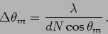 |
(12.23) |
Thus we see that the principal maxima get sharper as the number
of sources increases. Further, the th order maximum is the
sharpest, and the width of the maximum increases with increasing
order .
The chain of radiation sources serves as an useful model for many
applications.
Subsections
Next: Phased array
Up: Diffraction
Previous: Angular resolution
Contents
Physics 1st Year
2009-01-06