Resonance

As an example we consider a situation where the two particles are initially at rest in the equilibrium position. The particle $x_0$ is given a small displacement $a_0$ and then left to oscillate. Using this to determine $\tilde{A}_1$ and $\tilde{A}_2$, we finally have

$$x_0 (t) = \frac{a_0}{2} \left[ \cos \ \omega_0 t + \cos \ \omega_1 t \right]$$ (5.13)

and

$$x_1 (t) = \frac{a_0}{2} \left[ \cos \ \omega_0 t - \cos \ \omega_1 t \right]$$ (5.14)

The solution can also be written as

$$x_0(t) = a_0 \ \cos \left[\left( \frac{\omega_1 - \omega_0 ... ...ft[ \left( \frac{\omega_0 + \omega_1}{2} \right) t \right]$$ (5.15)

$$x_1(t) = a_0 \ \sin \left[ \left( \frac{\omega_1 - \omega_0... ...ft[ \left( \frac{\omega_0 + \omega_1}{2} \right) t \right]$$ (5.16)

It is interesting to consider $k'\ll k$ where the two oscillators are weakly coupled. In this limit

$$\omega_1 = \sqrt{\frac{k}{m} \left(1 + \frac{2 k'}{k} \right)} \approx \omega_0 + \frac{k'}{k} \omega_0$$ (5.17)

and we have solutions

$$x_0 (t) = \left[ a_0 \ \cos \left(\ \frac{k'}{2 k} \omega_0 t \right) \ \right] \cos \ \omega_0 t$$ (5.18)

and

$$x_1 (t) = \left[ a_0 \ \sin \left(\ \frac{k'}{2 k} \omega_0 t \right) \ \right] \sin \ \omega_0 t \,.$$ (5.19)

Figure 5.5: This shows the motion of $x_0$ and $x_1$.

The solution is shown in Figure 5.5. We can think of the motion as an oscillation with $\omega_0$ where the amplitude undergoes a slow modulation at angular frequency $\frac{k'}{2 k} \omega_0$. The oscillations of the two particles are out of phase and are slowly transferred from the particle which receives the initial displacement to the particle originally at rest, and then back again.

Problems

1. For the coupled oscillator shown in FIgure 5.1 with $k=10\, {\rm N}{\rm m}^{-1}$, $k'= 30 \, {\rm N}{\rm m}^{-1}$ and $m=1 \, {\rm kg}$, both particles are initially at rest. The system is set into oscillations by displacing $x_0$ by $40 \, {\rm cm}$ while $x_1=0$.

   [a.] What is the angular frequency of the faster normal mode? [b.] Calculate the average kinetic energy of $x_1$? [c.] How does the average kinetic energy of $x_1$ change if the mass of both the particles is doubled? ([a.] $8.37 \, {\rm s}^{-1}$ [b.] $8.00 \times 10^{-1} \, {\rm J}$ [c.] No change)

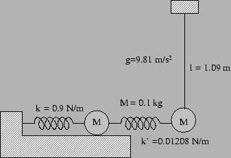
2. For a coupled oscillator with $k=8\, {\rm N}{\rm m}^{-1}$, $k'= 10 \, {\rm N}{\rm m}^{-1}$ and , both particles are initially at rest. The system is set into oscillations by displacing $x_0$ by $10 \, {\rm cm}$ while .

   [a.] What are the angular frequencies of the two normal modes of this system? [b.] With what time period does the instantaneous potential energy of the middle spring oscillate? [c.] What is the average potential energy of the middle spring?

3. Consider a coupled oscillator with $k=9\, {\rm N}{\rm m}^{-1}$, $k'= 8 \, {\rm N}{\rm m}^{-1}$ and $m=1 \, {\rm kg}$. Initially both particles have zero velocity with $x_0=10 \, {\rm cm}$ and $x_1=0$. [a.] After how much time does the system return to the initial configuration? [b.] After how much time is the separation between the two masses maximum? [c.] What are the avergae kinetic and potential energy? ([a.] $2 \pi \, {\rm s}$, [b.] $\pi/5 \, {\rm s}$ [c.] $14.25 \times 10^{-2} {\rm J}$)

4. A coupled oscillator has $k=9\, {\rm N}{\rm m}^{-1}$, $k'= 0.1 \, {\rm N}{\rm m}^{-1}$ and $m=1 \, {\rm kg}$. Initially both particles have zero velocity with $x_0=5 \, {\rm cm}$ and $x_1=0$. After how many oscillations in $x_0$ does it completely die down? (45)

5. Find out the frequencies of the normal modes for the following coupled pendula (see figure 5.6) for small oscillations. Calculate time period for beats.

   Figure 5.6: Problem 5 and 6

   

   

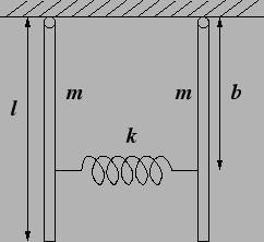6. A coupled system is in a vertical plane. Each rod is of mass $m$ and length $l$ and can freely oscillate about the point of suspension. The spring is attached at a length $b$ from the points of suspensions (see figure 5.6). Find the frequencies of normal(eigen) modes. Find out the ratios of amplitudes of the two oscillators for exciting the normal(eigen) modes.

7. Mechanical filter:Damped-forced-coupled oscillator- Suppose one of the masses in the system (say mass 1) is under sinusoidal forcing $F(t)=F_0\cos\omega t$. Include also resistance in the system such that the damping term is equal to $-2r\times {\rm velocity}$. Write down the equations of motion for the above system.

   Solution 7:
   

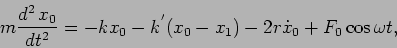   $$m \frac{d^2 \, x_0}{dt^2} = - k x_0 - k^{'} (x_0 - x_1) -2r{\dot{x}_0}+F_0\cos\omega t,$$ (5.20)

   
   
   
   

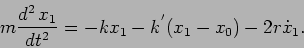   $$m \frac{d^2 \, x_1}{dt^2} = - k x_1 - k^{'} (x_1- x_0)-2r{\dot{x}_1}.$$ (5.21)

   
   

   Rearranging the terms we have (with notations of forced oscillations),

   
   

   $${\ddot{x}_0}+2\beta{\dot{x}_0}+\omega_0^2 x_0 +{{k^{'}}\over m} (x_0 - x_1) =f_0\cos\omega t,$$ (5.22)

   
   
   
   

   $${\ddot{x}_1}+2\beta{\dot{x}_1} +\omega_0^2 x_1 + {{k^{'}}\over m}(x_1-x_0)=0.$$ (5.23)

   
   

8. Solve the equations by identifying the normal modes.

   Solution 8: Decouple the equations using $q_0$ and $q_1$.
   

   
   
   
   

   $${\ddot{q}_1}+2\beta{\dot{q}_1} +\omega_1^2 q_1 ={{f_0}\over 2}\cos\omega t.$$ (5.25)

   
   

9. Write down the solutions of $q_0$ and $q_1$ as $q_0=z_0\cos\omega t$ and $q_1=z_1\cos\omega t$ respectively, with $z_0=\vert z_0\vert\exp(i\phi_0)$ and $z_1=\vert z_1\vert\exp(i\phi_1)$. Find $\vert z_0\vert,\phi_0,\vert z_1\vert$ and $\phi_1$.

10. Find amplitudes of the original masses, viz $x_0$ and $x_1$.
    
    $$x_0=q_0+q_1=z_0\cos\omega t+ z_1\cos\omega t=(z_0+z_1)\cos\omega t\equiv \vert A_0\vert\cos(\omega t +\Phi_0)$$
    
    
    
    
    $$x_1=q_0-q_1=z_0\cos\omega t- z_1\cos\omega t=(z_0-z_1)\cos\omega t\equiv \vert A_1\vert\cos(\omega t +\Phi_1)$$
    
    
    Do phasor addition and subtraction to evaluate amplitudes $\vert A_0\vert$ and $\vert A_1\vert$. Find also the the phases $\Phi_0$ and $\Phi_1$.

11. Using above results show that:

    
    

    $${{\vert A_1\vert^2}\over {\vert A_0\vert^2}}={{(\omega_1^2-\o... ...over {(\omega_1^2+\omega_0^2-2\omega^2)^2+16\beta^2\omega^2}}.$$
    
    

12. Plot the above ratio of amplitudes of two coupled oscillators as a function of forcing frequency $\omega$ using very small damping (i.e. neglecting the $\beta$ term). From there observe that the ratio of amplitudes dies as the forcing frequency goes below $\omega_0$ or above $\omega_1$. So the system works as a band pass filter, i.e. the unforced mass has large amplitude only when the forcing frequency is in between $\omega_0$ and $\omega_1$. Otherwise it does not respond to forcing.