Probability

Consider a process whose outcome is uncertain. For example, we throw a dice. The value the dice returns can have 6 values,

$$x_{_1}=1 ~~ x_{_2}=2 ~~ x_{_3}=3 ~~ x_{_4}=4 ~~ x_{_5}=5 ~~ x_{_6}=6$$ (19.1)

We can ask the question ``What is the probability of getting an outcome $x_i$ when you throw the dice?'' This probability can be calculated using,

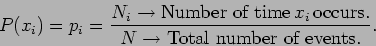$$P(x_i) = p_i=\frac{N_i \to \mbox{Number of time} \, x_i \, \mbox{occurs.}}{N \to \mbox{Total number of events.}}.$$ (19.2)

For a fair dice $P(x_i) = \frac{1}{6}$ for all the six possible outcomes as shown in Figure 19.1.

Figure 19.1: Probabilities of different outcomes for a fair dice

What is the expected outcome when we throw the dice? We next calculate the expectation value which again is an integral,

$$\langle x \rangle =$$ (19.3)

$$= \frac{21}{6} = \frac{7}{2} = 3.5.$$

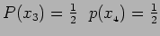Suppose we have a biased dice which produces only $3$ and $4$. We have $P(x_3) = \frac{1}{2} ~~ p(x_{_4}) = \frac{1}{2}$ , the rest are all zero as shown in Figure 19.2.

Figure 19.2: Probabilities of different outcomes for a biased dice

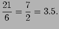
Calculating the expectation value for the biased dice we have

$$\langle x \rangle =3.5 \,.$$ (19.4)

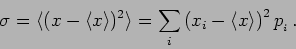
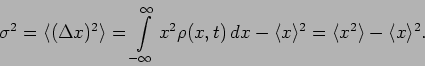
The expectation value is unchanged even though the probability distributions are different. Whether we throw the unbiased dice or the biased dice, the expected value is the same. Each time we throw the dice, we will get a different value . In both cases the values will be spread around 3.5 . The values will have a larger spread for the fair dice as compared to the biased one. How to characterize this? The root mean square or standard deviation $\sigma$ tells this. The variance $\sigma^2$ is calculated as,

$$\sigma = {\langle ( x- \langle x \rangle )^2 \rangle } = {\sum \limits_i \left( x_i - \langle x \rangle \right)^2 p_{_i}}\,.$$ (19.5)

Larger the value of $\sigma$ the more is the spread. Let us calculate the variance for the fair dice,

$$\sigma^2=\frac{1}{6} \left[ (1-3.5)^2+(2-3.5)^2+ ... + (6-3.5)^2 \right],$$ (19.6)

which gives the standard deviation $\sigma=1.7$. For the biased dice we have

$$\sigma^2=\frac{1}{2} \left[ (3-3.5)^2+(4-3.5)^2 \right],$$ (19.7)

which gives $\sigma=0.5$. We see that the fair dice has a larger variance and standard deviation then the unbiased one. The uncertainty in the outcome is larger for the fair dice and is smaller for the biased one.

We now shift over attention to continuous variables. For example, x is a random variable which can have any value between $0$ and $10$ (Figure 19.3). What is the probability that x has a value $2.36$ ?

Figure 19.3:

This probability is zero. We see this as follows. The probability of any value between 0 and 10 is the same. There are infinite points between $0$ and $10$ and the probability of getting exactly $2.36$ is,

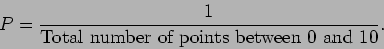$$P= \frac{1}{\mbox{Total number of points between 0 and 10}}.$$ (19.8)

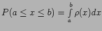
The denominator is infinitely large and the probability is thus zero. A correct question would be, what is the probability that $x$ has a value between and $2.36+0.001$. We can calculate this as,

$$\frac{2.361 - 2.359}{10.-0.} = 2 \times 10^{-4}.$$ (19.9)

For a continuous variable it does not make sense to ask for the probability of its having a particular value $x$. A meaningful question is, what is the probability that it has a value in the interval $\Delta x$ around the value $x$.

Making $\Delta x$ an infinitesimal we have,

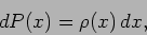$$dP(x) = \rho(x)\, dx,$$ (19.10)

where $d P$ is probability of getting a value in the internal $x- \frac{dx}{2}$ to $x+\frac{dx}{2}$. If all values in the range $0$ to $10$ are equally probable then,

$$\rho(x) = \frac{1}{10}.$$ (19.11)

The function $\rho(x)$ is called the probability density. It has the properties:

1. It is necessarily positive $\rho(x) \ge 0$
2. $P(a \le x \le b ) =\int \limits^b_a \rho(x) dx$ gives the probability that $x$ has a value in the range $a$ to $b$.
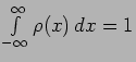
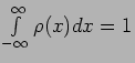3. $\int \limits^\infty_{-\infty}\rho (x) dx=1$ Total probability is

Let us consider an example (Figure 19.4) where

$$0 \le x \le \pi ~~ \rho(x) = A \sin^2 x,$$

$$\mbox{outside}\hspace{1.5cm} = 0.$$ (19.12)

Figure 19.4:

We first normalize the probability density. This means to ensure that $\int \limits_{-\infty}^{\infty} \rho(x) \, dx =1$. Applying this condition we have,

$$A \int \limits^\pi_0 \sin^2 x \, dx =$$

$$= \left. \frac{A}{2} \left[ \pi - \frac{1}{2} \sin (2x)\right\vert _0^\pi \right] = \frac{\pi A}{2} =1,$$ (19.13)

which gives us,

$$A = \frac{2}{\pi}.$$ (19.14)

We next calculate the expectation value $\langle x \rangle$. The sum in equation (19.3) is now replaced by an integral and,

$$\langle x \rangle = \int x \rho (x) dx.$$ (19.15)

Evaluating this we have,

$$\langle x \rangle= \frac{2}{\pi} \int \limits^\pi_0 x \sin^2 (x) dx = \frac{\pi}{2}.$$ (19.16)

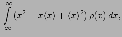
We next calculate the variance,

$$\sigma^2= \langle(x- \langle x \rangle)^2 \rangle = \int \limits^\infty_{-\infty} (x- \langle x \rangle)^2 \rho (x) dx.$$ (19.17)

This can be simplified as,

$$\sigma^2= = \int \limits^\infty_{-\infty} (x^2 - x \langle x \rangle + \langle x \rangle^2) \, \rho (x)\, dx,$$

$$=$$ (19.18)

Problem Calculate the variance $\sigma^2$ for the probability distribution in equation (19.12).

We now return to the wave $\psi(x,t)$ associated with every particle. The laws governing this wave are referred to as Quantum Mechanics. We have already learnt that this wave is to be interpreted as the probability amplitude. The probability amplitude can be used to calculate the probability density $\rho(x,t)$ using,

$$\rho (x,t) = \psi(x,t) \psi^{*}(x,t),$$ (19.19)

and

$$dP = \rho(x,t) \, dx,$$

gives the probability of finding the particle in an interval $dx$ around the point $x$. The expectation value of the particle's position can be calculated using,

$$\langle x \rangle = \int x \rho (x) \, dx \,.$$

This is the expected value if we measure the particle's position. Typically, a measurement will not yield this value. If the position of many identical particles all of which have the ``wave function'' $\psi(x,t)$ are measured these values will be centered around $\langle x \rangle$. The spread in the measured values of $x$ is quantified through the variance,

$$\sigma^2=\langle (\Delta x)^2 \rangle = \int \limits_{-\inft... ...\langle x \rangle^2= \langle x^2 \rangle -\langle x \rangle^2.$$ (19.20)

The standard deviation which is also denoted as $\Delta x \equiv \sqrt{\langle (\Delta x)^2 \rangle}=\sigma$ gives an estimate of the uncertainty in the particle's position.

Problems

1. The measurement of a particle's position $x$ in seven identical replicas of the same system we get values $1.3$, $2.1$, , $2,56$, $6.12$, $3.12$ and $9.1$. What are the expectation value and uncertainty in $x$?
2. In an experiment the value of $x$ is found to be different each time the experiment is performed. The values of $x$ are found to be always positive, and the distribution is found to be well described by a probability density
   
   $$\rho(x)=\frac{1}{L} \exp[-x/L] \hspace{1cm} L=0.2 \, {\rm m}$$
   
   

   a.

   What is the expected value of $x$ if the experiment is performed once?

   b.

   What is the uncertainty $\Delta x$?

   c.

   What is the probability that $x$ is less than $0.2 \, {\rm m}$?

   d.

   The experiment is performed ten times. What is the probability that all the values of $x$ are less than $0.2 \, {\rm m}$?

3. For a Gaussian probability density distribution
   
   
   

   a.

   Calculate the normalization coefficient $A$.

   b.

   What is the expectation value $\langle x \rangle$?

   c.

   What is the uncertainty $\Delta x = \sqrt{ \langle ( x-\langle x \rangle)^2 \rangle}$?

   d.

   What is the probability that $x$ has a positive value?