


Next: Transverse waves in stretched
Up: The wave equation.
Previous: The wave equation.
Contents
Figure 15.1:
An elastic beam
|
Consider a beam made of elastic material with
cross sectional area A as shown in Figure 15.1.
Lines have been shown at an uniform
spacing along the length of the beam .
Figure 15.2:
Compression and rarefaction in a disturbed beam
|
A disturbance is introduced in this beam as shown in
Figure 15.2. This also shows the undisturbed beam. The
disturbance causes the rod to be compressed at some places ( where
the lines have come closer ) and to get rarefied at some other
places ( where the lines have moved apart). The beam is made of
elastic material which tries to oppose the deformation i.e. the
compressed region tries to expand again to its original size and
same with the rarefied region. We would like to study the
behaviour of these disturbances in an elastic beam.
Let us consider the material originally at the point  of the
undisturbed beam (Figure15.2). This material is displaced to
of the
undisturbed beam (Figure15.2). This material is displaced to
 where
where
 is the horizontal displacement ofa the point
on the rod.
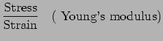
What happen to an elastic solid when it is compressed or extended?
is the horizontal displacement ofa the point
on the rod.
What happen to an elastic solid when it is compressed or extended?
Figure 15.3:
A rarefied section of the beam
|
|
Coming back to our disturbed beam, let us divide it into small
slabs of length  each. Each slab acts like a spring with
spring constant
each. Each slab acts like a spring with
spring constant
We focus our attention
to one particular slab ( shaded below ).
Figure 15.4:
One particular slab in the beam
|
|
Writing the equation of motion for this slab we have,
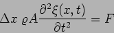 |
(15.4) |
where  is the density of the rod,
 the mass of the slab,
 its acceleration. F
denotes the total external forces acting on this slab.
its acceleration. F
denotes the total external forces acting on this slab.
The external forces arise from the adjacent slabs which are like
springs.
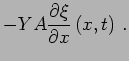
This force from the spring on the left is
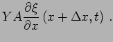
The force from the spring on the right is
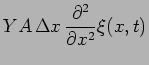
The total force acting on the shaded slab  is
is
Using this in the equation of motion of the slab (eq. 15.4) we
have
which gives us
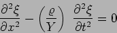 |
(15.12) |
This is a wave equation. Typically the wave equation is written as
where  is the phase velocity of the wave.
In this case
is the phase velocity of the wave.
In this case
In three dimensions the wave equation is
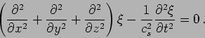 |
(15.14) |
This is expressed in a compact notation as
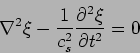 |
(15.15) |
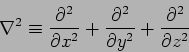
where  denotes the Laplacian operator defined as
We next check that the familiar sinusoidal plane wave discussed
earlier
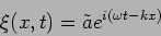 |
(15.16) |
is a solution of the wave equation. Substituting this in the wave
equation (15.15) gives us
 |
(15.17) |
Such a relation between the wave vector  and the angular
frequency
and the angular
frequency  is called a dispersion relation. We have
 |
(15.18) |
which tells us that the constant which appears in the wave
equation is the phase velocity of the wave.
Next: Transverse waves in stretched
Up: The wave equation.
Previous: The wave equation.
Contents
Physics 1st Year
2009-01-06


![\scalebox{0.6}{\includegraphics[angle=0,width=0.7\textwidth]{chapt15//p3.eps}}](img1163.png)