Single slit Diffraction Pattern.

Figure 12.3: Single slit diffraction

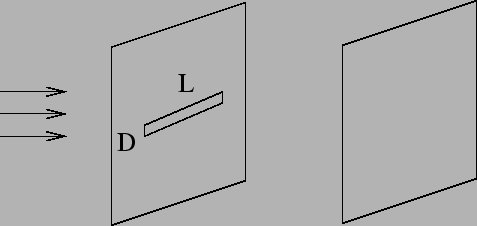
Consider a situation where light from a distant source falls on a rectangular slit of width $D$ and length $L$ as shown in Figure 12.3. We shall assume that $L$ is much larger than $D$. We are interested in the image on a screen which is at a great distance from the slit.

As the source is very far away, we can treat the incident light as plane wave. Further the source is aligned so that the incident wavefronts are parallel to the plane of the slit. Every point in the slit emits a spherical secondary wavelet.These secondary wavelets are well described by plane waves by the time they reach the distant screen. This situation where the incident wave and the emergent secondary waves can all be treated as plane waves is referred to as Fraunhofer diffraction. In this case both, the source as well as the screen are effectively at infinity from the obstacle.

Figure 12.4: Single slit effective one dimensional arrangement

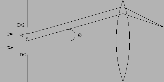
We assume L to be very large so that the problem can be treated as one dimensional as shown in Figure 12.4. Instead of placing the screen far away, it is equivalent to introduce a lens and place the screen at the focal plane. Each point on the slit acts like a secondary source. These secondary sources are all in phase and they all emit secondary wavelets with the same phase. Let us calculate the total radiation at a point at an angle $\theta$. If

$$d \tilde E = \tilde A ~ dy$$ (12.1)

be the contribution from a small element dy at the center of the slit, the contribution from an element a distance $y$ away will be at a different phase

$$d \tilde E = \tilde A ~ e^{i \delta} dy$$ (12.2)

where

$$\delta = \frac{2 \pi}{\lambda} y \sin \theta = ky$$ (12.3)

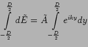
The total electric field can be calculated by adding up the contribution from all points on the slit. This is an integral

$$\tilde E = \int\limits^{\frac{D}{2}}_{-\frac{D}{2}} d \tilde E = \tilde A \int \limits^{\frac{D}{2}}_{-\frac{D}{2}} e^{iky} dy$$

$$= \tilde{A}D \sin \left(\frac{ kD}{2}\right) \, \left(\frac{kD}{2} \right)^{-1} = \tilde{A}D \, \mbox{sinc} \left(\frac{ kD}{2}\right)$$ (12.4)

where $\mbox{sinc}(x)=\sin(x)/x$. We use eq. (12.4) to calculate the intensity of light at an angle $\theta$. Defining

$$\beta = \frac{\pi D \, \sin \theta }{\lambda }\,,$$ (12.5)

the intensity is given by

$$I(\beta) = \frac{1}{2} EE^* = I_0 \, \mbox{sinc}^2 \beta \, .$$ (12.6)

Figure 12.5: Single slit intensity pattern

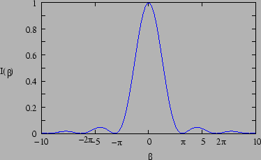
Figure 12.5 shows the intensity as a function of $\beta$. The intensity is maximum at the center where $\beta=0$. In addition to the oscillations, the intensity falls off proportional to $\beta^2$ away from the center. The analysis of the intensity pattern is further simplified In the situation where $\theta \ll 1$ as

$$\beta = \frac{\pi D \, \theta }{\lambda }\,.$$ (12.7)

The zeros of the intensity pattern occur at $\beta= \pm m \pi ~~ (m,= 1, 2,3,\ldots)$, or in terms of the angle $\theta$, the zeros are at

$$\theta = m \frac{\lambda}{D} \,.$$ (12.8)

There are intensity maxima located between the zeros. The central maximum at $\theta = 0$ is the brightest, and its angular separation from the nearest zero is $\lambda/D$. This gives an estimate of the angular width of the central maximum. The intensities of the other maxima fall away from the center.

Let us compare the intensity pattern $I(\beta)$ shown in Figure 12.5 with the predictions of geometrical optics. Figure 12.4 shows a beam of parallel rays incident on a slit of dimension $D$. In geometrical optics the only effect of the slit is to cut off some of the rays in the incident beam and reduce the transverse extent of the beam. We expect a beam of parallel rays with transverse dimension $D$ to emerge from the slit. This beam is now incident on a lens which will focuses all the rays to a single point on the screen. Thus in geometrical optics the image is a single bright point on the screen. In reality the wave nature of light manifests itself through the phenomena of diffraction, and we see a pattern of bright spots as shown in Figure 12.5. The central spot is the brightest and it has an angular extent The other spots located above and below the central spot are fainter. Taking into account both dimensions of the slit we have

(12.9)

where

$$\beta_x = \frac{\pi L \theta_x }{\lambda} \hspace{1cm} \mb... ...d} \hspace{1cm} \beta_y = \frac{\pi D \theta_y }{\lambda} \,.$$ (12.10)

and $\theta_x$ and $\theta_y$ are the angles along the $x$ and $y$ axis respectively. The diffraction effects are important on angular scales $\theta_x \sim \lambda/L$ and $\theta_y \sim \lambda/D$. In the situation where $L \gg D$ the diffraction effects along $\theta_x$ will not be discernable , and we can treat it as a one dimensional slit of dimension $D$.