Next: Diffraction
Up: Coherence
Previous: Spatial Coherence
Contents
The Michelson interferometer measures the temporal coherence of
the wave. Here a single wave front  is split into two
 and
and
 at the beam splitter. This is referred to
as division of amplitude. The two waves are then superposed, one
of the waves being given an extra time delay
at the beam splitter. This is referred to
as division of amplitude. The two waves are then superposed, one
of the waves being given an extra time delay  through the
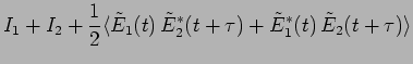
difference in the arm lengths. The intensity of the fringes is
through the
difference in the arm lengths. The intensity of the fringes is
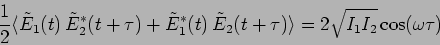
where it is last term involving
 which is responsible for interference.
In our analysis of the Michelson interferometer in the previous chapter
we had assumed that the incident wave is purely monochromatic ie.
which is responsible for interference.
In our analysis of the Michelson interferometer in the previous chapter
we had assumed that the incident wave is purely monochromatic ie.
 whereby
 |
(11.10) |
The above assumption is an idealization that we adopt because it
simplifies the analysis. In reality we do not have waves of a single
frequency, there is always a finite spread in frequencies. How does
this affect eq. 11.10?
As an example let us consider two frequencies
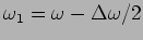 and
and
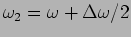 with
with

![\begin{displaymath}
\tilde{E}(t)=\tilde{a}\left[ e^{i \omega_1 t} + e^{i \omega_2 t} \right]\,.
\end{displaymath}](img898.png) |
(11.11) |
This can also be written as
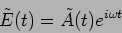 |
(11.12) |
which is a wave of angular frequency  whose amplitude
varies slowly with time.
We now consider a more realistic situation where we have many
frequencies in the range
whose amplitude
varies slowly with time.
We now consider a more realistic situation where we have many
frequencies in the range
 to
to
 . The resultant will again be of the same
form as eq. (11.12) where there is a wave with angular
frequency whose
amplitude
. The resultant will again be of the same
form as eq. (11.12) where there is a wave with angular
frequency whose
amplitude  varies slowly on the timescale
Figure 11.4:
Variation of E
with time for monochromatic and polychromatic light
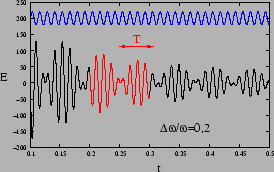 |
Note that the amplitude  and phase
  of the complex
amplitude both vary slowly with timescale T.
Figure 11.4 shows a situation where
of the complex
amplitude both vary slowly with timescale T.
Figure 11.4 shows a situation where
 , a pure sinusoidal wave of the same frequency
is shown for comparison. What happens to eq. (11.10) in
the presence of a finite spread in frequencies? It now gets
modified to
, a pure sinusoidal wave of the same frequency
is shown for comparison. What happens to eq. (11.10) in
the presence of a finite spread in frequencies? It now gets
modified to
 |
(11.13) |
where
 . Here
  is the temporal
coherence of the two waves
and
for a time delay
.
Two waves are perfectly coherent if
, partially
coherent if
is the temporal
coherence of the two waves
and
for a time delay
.
Two waves are perfectly coherent if
, partially
coherent if
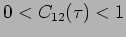 and incoherent if
 .
Typically the coherence time
.
Typically the coherence time  of a wave is decided by the
spread in frequencies
of a wave is decided by the
spread in frequencies
The waves are coherent for time delays less than
ie.
 for
for  , and the waves are
incoherent for larger time delays ie.
, and the waves are
incoherent for larger time delays ie.
 for
for
 . Interference will be observed only if .
The coherence time can be converted to a
length-scale
. Interference will be observed only if .
The coherence time can be converted to a
length-scale  called the coherence length.
An estimate of the frequency spread
 can be made by studying the intensity distribution of
a source with respect to frequency. Full width at half maximum
(FWHM) of the intensity profile gives a good estimate of the
frequency spread.
can be made by studying the intensity distribution of
a source with respect to frequency. Full width at half maximum
(FWHM) of the intensity profile gives a good estimate of the
frequency spread.
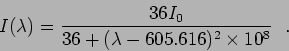
The Michelson interferometer can be used to measure the temporal
coherence . Assuming that  , we have
 . Measuring the visibility of the fringes varying
 the difference in the arm lengths of a Michelson
interferometer gives an estimate of the temporal coherence for
the difference in the arm lengths of a Michelson
interferometer gives an estimate of the temporal coherence for
 . The fringes will have a good contrast
  only
for
only
for  . The fringes will be washed away for values
larger than
. The fringes will be washed away for values
larger than  .
.
Problems
- Consider a situation where Young's double slit experiment is
performed using light of wavelength
 and
and
 . Calculate the visibility assuming a source of angular
width
. Calculate the visibility assuming a source of angular
width  and . Plot
  for both these
cases.
for both these
cases.
- A small aperture of diameter
 at a distance of
 is used to illuminate two slits with light of wavelength
 . The slit separation is
 . What is the fringe spacing and the expected visibility of the
fringe pattern? (
. What is the fringe spacing and the expected visibility of the
fringe pattern? (
 ,
,  )
)
- A source of unknown angular extent
 emitting light at
is used in a Young's
double slit experiment where the slit spacing can be varied. The
visibility is measured for different values of . It is found
that the fringes vanish
emitting light at
is used in a Young's
double slit experiment where the slit spacing can be varied. The
visibility is measured for different values of . It is found
that the fringes vanish  for
for
 . [a.] What is
the angular extent of the source? (
. [a.] What is
the angular extent of the source? (
 )
)
- Estimate the coherence time and coherence length
for the following sources
| Source |
 nm nm |
 nm nm |
| White light |
550 |
300 |
| Mercury arc |
546.1 |
1.0 |
| Argon ion gas laser |
488 |
0.06 |
| Red Cadmium |
643.847 |
0.0007 |
| Solid state laser |
785 |
 |
| He-Ne laser |
632.8 |
 |
- Assume that Kr
 discharge lamp has roughly the
following intensity distribution at various wavelengths,
(in
discharge lamp has roughly the
following intensity distribution at various wavelengths,
(in  ),
),
Estimate the coherence length of Kr source.(Ans. 0.3m)
- An ideal Young's double slit (i.e. identical slits with
negligible slit width) is illuminated with a source having two
wavelengths,
 and
and
 . The
intensity at
. The
intensity at  is double of that at
  .
.
a) Compare the visibility of fringes near order  and near
order
and near
order  on the screen [visibility =
 ].(Ans. 1:0.5)
b) At what order(s) on the screen visibility of the fringes is
poorest and what is this minimum value of the visibility. (Ans.
75, 225 etc. and 1/3)
- An ideal Young's double slit (separation between the
slits) is illuminated with two identical strong monochromatic
point sources of wavelength . The sources are placed
symmetrically and far away from the double slit. The angular
separation of the sources from the mid point of the double slit is
 . Estimate so that the visibility of the
fringes on the screen is zero. Can one have visibility almost 1
for a non zero .
. Estimate so that the visibility of the
fringes on the screen is zero. Can one have visibility almost 1
for a non zero .
Hint: See the following figure 11.5,
Figure 11.5:
Two source
vanishing visibility condition
|
(Further reading: Michelson's stellar interferometer for
estimating angular separation of double stars and diameters of
distant stars)
Next: Diffraction
Up: Coherence
Previous: Spatial Coherence
Contents
Physics 1st Year
2009-01-06
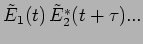
![$\displaystyle \frac{1}{2} \langle [\tilde{E}_1(t)+\tilde{E}_2(t+\tau)] \, [\tilde{E}_1(t)+\tilde{E}_2(t+\tau)]^*
\rangle$](img891.png)