Next: Resonance.
Up: Oscillator with external forcing.
Previous: Complementary function and particular
Contents
Introducing damping, the equation of motion
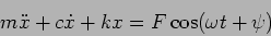 |
(3.12) |
written using the notation introduced earlier is
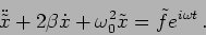 |
(3.13) |
Here again we separately discuss the complementary functions and the
particular integral. The complementary functions are the decaying
solutions that arise when there is no external force.
These are short lived transients which are not of interest when
studying the long time behaviour of the oscillations. These have
already been discussed in considerable detail and we do not consider
them here.
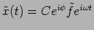
The particular integral
is important when studying the long time or steady state
response of the oscillator. This solution is
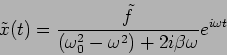 |
(3.14) |
which may be written as
 where
where
 is the phase of the oscillation relative to the force
  .
.
This has an amplitude
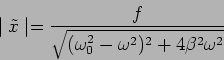 |
(3.15) |
and the phase is
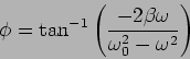 |
(3.16) |
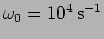
Figure 3.2:
Amplitudes and phases for various damping coefficients as a function of
driving frequency
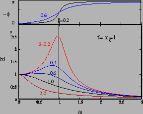 |
Figure 3.2 shows the amplitude and phase as a function of
 for different
values of the damping coefficient
for different
values of the damping coefficient  . The damping ensures that
the amplitude does not blow up at
. The damping ensures that
the amplitude does not blow up at
 and it
is finite for all values of . The change in
the phase also is more gradual.
and it
is finite for all values of . The change in
the phase also is more gradual.
The low frequency and high frequency behaviour are exactly the
same as the situation without damping. The changes due to damping are
mainly
in the vicinity of
. The amplitude is maximum at
 |
(3.17) |
For mild damping (
 ) this is approximately
.
) this is approximately
.
We next shift our attention to the energy of the oscillator. The average
energy  is the quantity of interest. Calculating this as a function of
we have
is the quantity of interest. Calculating this as a function of
we have
![\begin{displaymath}
E(\omega)={{m}f^2\over 4}{{(\omega^2+\omega_0^2)}\over
{[(\omega_0^2-\omega^2)^2+4\beta^2\omega^2]}}
\end{displaymath}](img267.png) |
(3.18) |
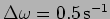
Figure 3.3:
Energy resonance
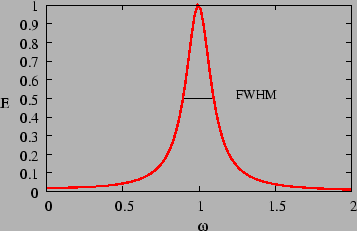 |
The response to the external force shows a
prominent peak or resonance (Figure 3.3) only when
, the mild damping limit. This is of
great utility in modelling the phenomena of resonance which occurs in
a large variety of situations. In the weak damping limit
peaks at
 and falls rapidly away from the
peak. As a consequence we can use
and falls rapidly away from the
peak. As a consequence we can use
 |
(3.19) |
which gives
![\begin{displaymath}
E(\omega) \approx \frac{k}{8}
\frac{f^2}{\omega_0^2[(\omega_0-\omega)^2 + \beta^2 ]}
\end{displaymath}](img271.png) |
(3.20) |
in the vicinity of the resonance.
This has a maxima at
and the maximum value
is
We next estimate the width of the peak or resonance. This
is quantified using the FWHM (Full Width at Half Maxima)
defined as FWHM =
 where
where
 ie. half the maximum value.
Using equation (3.20) we see that
ie. half the maximum value.
Using equation (3.20) we see that
 and FWHM
  .
as shown in Figure 3.3.
The FWHM quantifies the width of the curve and it records the fact
that the width increases with the damping coefficient .
.
as shown in Figure 3.3.
The FWHM quantifies the width of the curve and it records the fact
that the width increases with the damping coefficient .
The peak described by equation (3.20) is referred to as a
Lorentzian profile. This is seen in a large variety of situations
where we have a resonance.
We finally consider the power drawn by the oscillator from the
external force. The instantaneous power
 has a value
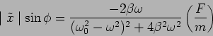
![\begin{displaymath}
P(t)= [F \cos(\omega t)] [- \mid \tilde{x}\mid \omega \sin(\omega t + \phi)] \,.
\end{displaymath}](img278.png) |
(3.22) |
The average power is the quantity of interest, we study this as a
function of the frequency. Calculating this we have
Using equation (3.14) we have
 |
(3.24) |
which gives the average power
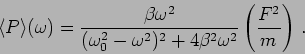 |
(3.25) |
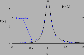
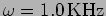
The solid curve in Figure 3.4 shows the average power as a
function of
.
Here again, a prominent, sharp peak is seen
only if
. In the mild damping limit, in the
vicinity of the maxima we have
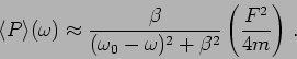 |
(3.26) |
which again is a Lorentzian profile. For comparison we have also plotted
the Lorentzian profile as a dashed curve in Figure
3.4.
Figure 3.4:
Power resonance
 |
Problem 1: Plot the response,  , of a forced oscillator with a forcing
 and natural frequency
  Hz with initial conditions,
 and
and  , for two different resistances,
  and
and
 . Plot also for fixed resistance, and different forcing
amplitudes
. Plot also for fixed resistance, and different forcing
amplitudes  and 9.
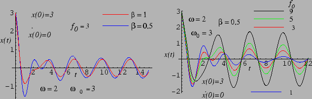
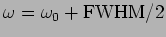
Solution 1: The evolution is shown in the Fig. 3.5. Notice that
the transients die and the steady state is achieved relatively sooner in the case
of larger resistance, . Furthermore, the steady state is reached quicker
in the case of larger forcing amplitude. See the variation of steady state
amplitudes for different parameters.
Figure 3.5:
Forced oscillations with different resistances and forcing amplitudes
 |
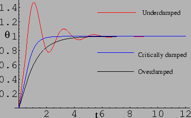
Problem 2: The galvanometer:
A galvanometer is connected with a constant-current
source through a switch. At time t=0, the switch is closed. After some time
the galvanometer deflection reaches its final
value  . Taking damping torque
proportional to the angular velocity draw deflection of the
galvanometer from the initial
position of rest (i.e.
. Taking damping torque
proportional to the angular velocity draw deflection of the
galvanometer from the initial
position of rest (i.e.  ,
,
 ) to its final position
 , for the underdamped, critically damped and overdamped
cases.
, for the underdamped, critically damped and overdamped
cases.
Solution 2: We solve the forced oscillator equation with constant
forcing (i.e. driving frequency =0)
and given initial conditions and plot the various evolutions. Figure 3.6
shows the galvanometer deflection as a function of time for some arbitrary values
of , damping coefficient and natural frequency.
Figure 3.6:
Galvanometer deflection
 |
Problems
- An oscillator with
 and negligible
damping is driven by an external force
and negligible
damping is driven by an external force
 .
By what percent do the amplitude of oscillation and the energy
change if is changed from
.
By what percent do the amplitude of oscillation and the energy
change if is changed from
 to
to
 ? (
? (
 )
)
- An oscillator with
 and
and
 is driven by an external force
.
[a.] Determine
is driven by an external force
.
[a.] Determine  where the power drawn by the oscillator
is maximum?
[b.] By what percent does the power fall if is changed by
where the power drawn by the oscillator
is maximum?
[b.] By what percent does the power fall if is changed by
 from ?[c.] Consider
 instead of
. (
([a.]
,
instead of
. (
([a.]
,  ,
,  )
)
- A mildly damped oscillator driven by an external force is known
to have a resonance at an angular frequency somewhere near
 with a quality factor of
  .
Further, for the force (in Newtons)
.
Further, for the force (in Newtons)
the amplitude of oscillations is  at
at
 and
and  at
at
 .
.
- a.
- What is the spring constant of the oscillator?
- b.
- What is the natural frequency
 of the oscillator?
- c.
- What is the FWHM?
- d.
- What is the phase difference between the force and the
oscillations at
 ?
?
- Show that,
 , is a solution of the undamped forced system,
, with initial conditions,
. Show that near resonance,
, is a solution of the undamped forced system,
, with initial conditions,
. Show that near resonance,
 ,
,
 , that is the amplitude of
the oscillations grow linearly with time. Plot the solution near resonance.
(Hint: Take
, that is the amplitude of
the oscillations grow linearly with time. Plot the solution near resonance.
(Hint: Take
 and expand the solution taking
 .)
.)
- Find the driving frequencies corresponding to the half-maximum power
points and hence find the FWHM for the power curve of Fig. 3.4.
- Show that the average power loss due to the resistance
dissipation is equal to the average input power calculated in the expression
(3.25).
- (a) Evaluate average energies at frequencies,
 (at the amplitude resonance) and
 (at the power resonance). Show that
they are equal and independent of .
(at the power resonance). Show that
they are equal and independent of .
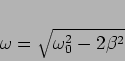
(b) Find the value of the forcing frequency,
, for which the
energy of the oscillator is maximum.
(c) What is the value of the maximum energy?
((a)  ,
,
(b)
 ,
,
 ,
,
(c)
 .)
.)
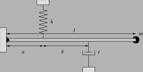
- A massless rigid rod of length
 is hinged at one end on the wall.
(see figure). A vertical spring of stiffness
is hinged at one end on the wall.
(see figure). A vertical spring of stiffness  is attached at a distance
  from the hinge. A damper is fixed at a further distance of
  from the spring
providing a resistance proportional to the velocity of the attached point of the
rod. Now a mass
from the spring
providing a resistance proportional to the velocity of the attached point of the
rod. Now a mass
 is plugged at the other end of the rod. Write
down the condition for critical damping (treat all angular displacements small).
If mass is displaced
is plugged at the other end of the rod. Write
down the condition for critical damping (treat all angular displacements small).
If mass is displaced  from the horizontal,
write down the subsequent motion of the mass for the above condition.
from the horizontal,
write down the subsequent motion of the mass for the above condition.
- A critically damped oscillator has mass 1 kg and the spring constant
equal to 4 N/m. It is forced with a periodic forcing
 N. Write the steady state solution for the oscillator. Find the average power per
cycle drawn from the forcing agent.
N. Write the steady state solution for the oscillator. Find the average power per
cycle drawn from the forcing agent.
- A horizontal spring with a stiffness constant
 N/m is fixed
on one end to a rigid wall. The other end of the spring is attached with
a mass of
N/m is fixed
on one end to a rigid wall. The other end of the spring is attached with
a mass of  kg resting on a frictionless horizontal table. At
  , when
the spring -mass system is in equilibrium and is perpendicular to the
wall, a force
, when
the spring -mass system is in equilibrium and is perpendicular to the
wall, a force  N
starts acting on the mass in a direction perpendicular to the
wall. Plot the displacement of the mass from the
equilibrium position between and
N
starts acting on the mass in a direction perpendicular to the
wall. Plot the displacement of the mass from the
equilibrium position between and  neatly.
Next: Resonance.
Up: Oscillator with external forcing.
Previous: Complementary function and particular
Contents
Physics 1st Year
2009-01-06